|
Sub-problem 3a - Page 8 of 13 |
ID# C403A08 |
Sub-problem 3a: Weaving Analysis
 |
|
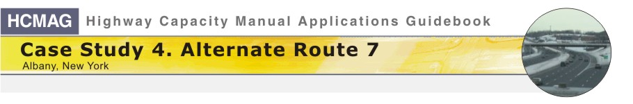
Exhibit 4-49. Scenario 1 weaving diagram
|
 |
|
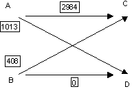
Exhibit 4-50. Scenario 2 weaving diagram
|
 |
|
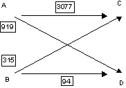
Exhibit 4-51. Scenario 3 weaving diagram
|
In this situation, we
can test the sensitivity of the results to the estimate we make about the
weaving movement volumes and show some common assumptions that are made in
such situations using three scenarios.
In the first
scenario, we assume that all the 23rd street on-ramp traffic goes
to I-787 north. This maximizes the weaving volumes. The weaving diagram for
this scenario is shown in Exhibit 4-49.
For the second
scenario, we’ll assume that the inbound flows go to the outbound legs
proportional to the exiting volumes. Since the volumes at C and D are 3,992
and 1,013, respectively, 77% of the exiting traffic from both of the
entering flows will go to C and 23% will go to D. This means the flow from A
to C is 3,075 veh/hr (77% of 3,992) and the flow from A to D is 920 veh/hr
(23% of 3,992). It also means the flow from B to C is 315 veh/hr and the
flow from B to D is 95 veh/hr. The resulting weaving diagram is shown in Exhibit
4-50.
For the third
scenario, we assume a larger percentage going to D from B, namely 40%. This
reduces the amount of traffic from A going to D. Thus, the weaving traffic
decreases and the non-weaving traffic increases. The weaving diagram for
this scenario is shown in Exhibit 4-51.
Exhibit
4-52 presents the results for these three scenarios You can see
that the density is greatest in Scenario 1, where the weaving volumes are
the largest. The density is lower in Scenario 2, where only 77% of the
vehicles getting on at B are assumed to go to C; and it’s the lowest in
Scenario 3, where 40% of the flow from B goes to D. As the weaving volumes
get smaller, the density should decrease.