Problem 5: Network Simulation

Printable Version

This problem demonstrates how a network simulation model can be used to augment studies conducted with HCM methodologies. Simulation models offer the advantage of being able to examine networks of highway facilities in a highly unified, holistic fashion. Inter-dependencies and cascading effects can be taken into account as can traffic variations of time, over saturation, queue length fluctuations, lane blockages, and other transient phenomena. The only major drawback is that simulation models are typically data-hungry and they take time to develop, debug, calibrate, validate, and run. Distilling the results also takes time, because there’s so much information to study, absorb, and comprehend.

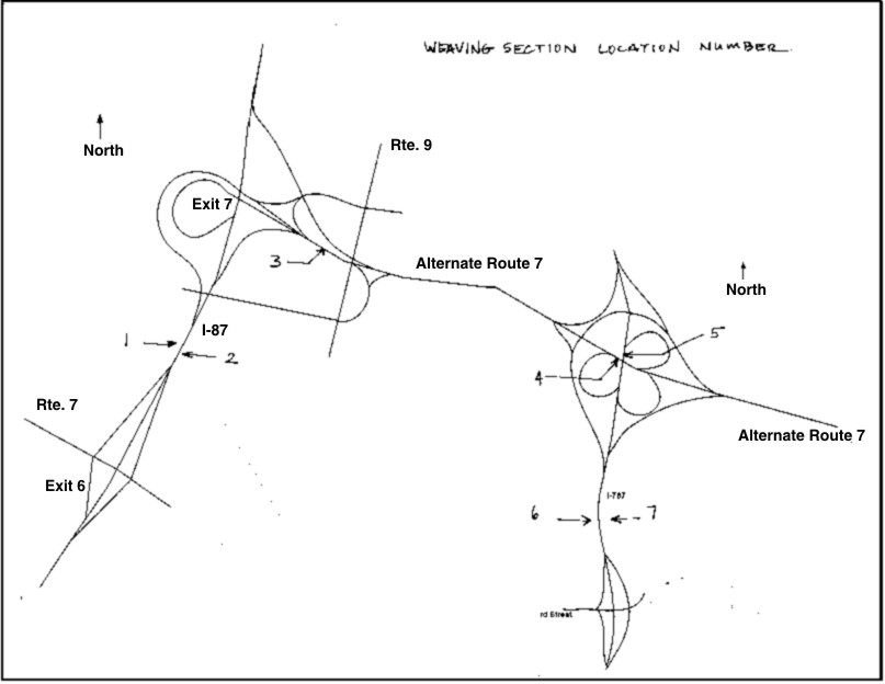
Two main decisions need to be made: 1) what network to analyze and 2) what traffic volumes to use. Exhibit 4-77 shows the network used as the basis for the simulation model. It encompasses Alternate Route 7 and the interchange complexes at either end: Exits 6 and 7 on I-87, the interchange with Route 9 on Route 7, and the interchanges with Route 7 and 23rd Street on I-787. What it doesn’t include is the underlying surface arterial network and the freeways that lie outside the artificially defined boundary. The actual simulation network is detailed, with information about lane configurations, vertical and horizontal geometry, speed limits, etc.

The time period we studied was the AM peak. Either the AM peak or the PM peak would be a good choice. The only difference is the direction of peak flow. In the AM Peak, the flows are predominantly southbound and eastbound.

Discussion:
Take a few minutes to consider these questions. When you are ready to continue, click continue below to proceed.

Sub-problem 5a: Network Simulation

Step 1. Setup

VISSIM is the traffic simulation package we chose to use, so the specific input data files reflect the needs of that software. However, many of these characteristics and inputs would be required for other modeling software as well. A summary of the inputs and assumptions we used is as follows:

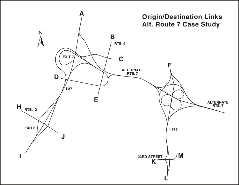
The O-D trip matrix was obtained from the Capital District Transportation Committee (CDTC), which serves as the local MPO. The matrix is derived from the outputs of the travel forecasting model that CDTC uses in all of its planning studies. Since it is generated data rather than observed volumes, we do not expect exact matches between the traffic volumes observed in the field and those predicted by the O-D trip matrix. The traffic volume on a given link in a given time period predicted by the O-D trip matrix may be different from the value that was actually observed in the field. The difference is that the predicted value uses a routing algorithm to assign flows to network paths that might not be consistent with the way drivers choose routes.

Consider:

Discussion:
Take a few minutes to consider these questions. Click continue when you are ready to proceed.

Sub-problem 5a: Network Simulation

Step 2. Results

The most interesting result from the simulation model is predictions of travel times through the network. Exhibit 4-79 presents a selected set of those values. You can see that it takes 467 seconds (seven minutes and 47 seconds) to go from a point 300 feet south of the 23^rd Street off- ramp to a point 2,600 feet north of the merge between I-87 and the right-hand ramp from NY-7 to I-87. These values are valuable in indicating where travel times are within acceptable ranges and where they are not. Geometric improvements may help some O-D pairs and not others or alleviate congestion in one place and create it in another. These travel times help to keep track of those impacts and relationships.

Another output that’s particularly valuable is speeds through the weaving sections. Weaving sections tend to be bottleneck locations. Exhibit 4-80 shows speeds for weaving and non-weaving vehicles at a number of locations in the subarea network, based on the simulation model outputs. Data for locations 1-7 are shown in Exhibit 4-80. The slowest speeds are on Alternate Route 7 at the I-787 interchange on the collector-distributor road between the loop ramp from I-787 south and the loop ramp to I-787 north. The rest of the speeds are in the 50-60 mph range, indicating acceptable operation.

Sub-problem 5a: Network Simulation

Discussion
Probably the most significant lesson learned from Problem 5 is that it is possible to develop a simulation model for the subarea network. We also learned that it is possible to obtain interesting pieces of information about the performance of the network to help planners and designers understand where there are problems and what can be done about them.

The simulation model is a diagnostic tool, not a solution generator. It can tell how a given network configuration performs and let you compare and contrast one solution with another. The model won’t tell where to add capacity or how much. These need to be obtained through engineering judgment or trial and error. But you have to develop the solution ideas.