Problem 3: Basic Freeway Sections

Printable Version

Figure 2-1 contains a diagrammatic picture of the interchange complex on the eastern end of Alternate Route 7. As can be seen, the Rte-7/I-787 interchange is basically a cloverleaf with one semi-direct ramp. Originally, the plan was to have I-787 continue eastward, through Troy, and overlap the Rte-7 alignment to the Vermont border. The idea was squelched when it became clear that the freeway alignment through Troy would involve taking many homes and effectively closing Hoosick Street, a major arterial.

Consistent with Table 1 in the introduction, Figure 2-1 also shows the locations where specific analyses will be focused:

1. Eastbound weave on Rte-7 as it crosses the Hudson River.

2. Westbound weave on Rte-7 as it crosses the Hudson River.

3. Northbound weave on I-787 between the 23^rd street interchange and the Rte 7 interchange

4. Southbound weave on I-787 between the 23^rd street interchange and the Rte 7 interchange

5. Northbound weave on I-787 between the loop ramps

6. Eastbound diverge on Rte 7 that leads to both the right-hand ramp to I-787 and the auxiliary lane that connects to the loop ramps to and from I-787

7. Southbound merge between the right-hand ramp coming from Rte 7 east and the semi-direct loop ramp coming from Rte 7 west.

8. Southbound merge between the combined ramp from G above and I-787 south.

9. Westbound merge between Rte 7 and the loop ramp coming from I-787 north.

10. Westbound merge between Rte 7 and the right-hand ramp coming from I-787 south.

11. Eastbound merge between the auxiliary eastbound lane on Rte 7 and the loop ramp coming from I-787 southbound.

12. Eastbound diverge involving the auxiliary eastbound lane on Rte 7 and the loop ramp leading to I-787 northbound.

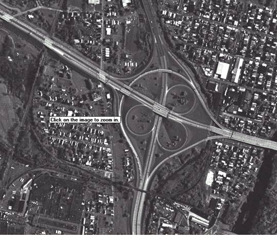
 [ Back ] [ Continue ] with Problem 3

Problem 3: Basic Freeway Sections

Figure 2 contains an aerial photograph of the I-787 interchange. You can see the three loop ramps, the four right-hand ramps, and the semi-direct ramp leading from Rte 7 westbound to I-787 southbound. You can also see the auxiliary lane on the south side of eastbound lanes that starts with the right-hand ramps extends through the two loop ramps and then reunites with the eastbound lanes just east of the east-to-north loop ramp. The short northbound weaving section under the Rte 7 bridges is plainly apparent as is the tight radius that is part of the right-hand ramp leading from Rte 7 eastbound to I-787 southbound.

Figure 2. Aerial Photograph of the I-787 Interchange

 [ Back ] [ Continue ] with Problem 1

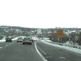
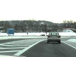
Problem 3: Basic Freeway Section

Figure 3 shows a view of Rte 7 at location F looking eastbound toward Troy. You can see the beginning of the auxiliary lane that leads to the right-hand ramp and the loop ramps. In the background, you can see the signs for the loop ramp to I-787 north and the merge sign for the place where the auxiliary lane rejoins Route 7 east.

Figure 4 shows a view of location G where the right-hand ramp from Route 7 east to I-787 south merges with the semi-direct ramp coming from Rte 7 west. You can see the semi-direct ramp from Rte 7 east to the left of the vehicle ahead and you can tell that the two single lane ramps are about to merge not far downstream.

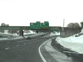
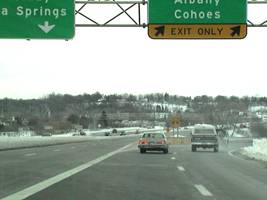
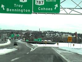
 [ Back ] [ Continue ] with Problem 3

Problem 3: Basic Freeway Sections

Figure 5 shows a view of Location C looking north, just before the double-lane right-hand ramp leaves to head toward Rte 7 east. You can see the two lanes of I-787 that continue north under the railroad bridge and then Route 7. You can also see the signs for Route 7 east on the right (leading toward Troy) and Route 7 west (leading toward Saratoga Springs). The truck in the distance at the front of the platoon traveling north on I-787 is at the beginning of the weaving section designated as Location E in Figure Figure 1.

Figure 6 shows a view of Rte 7 west just at the end of the weaving section designated as Location A in Figure 2-1. You can see the beginning of the semi-direct ramp leading from Rte 7 west toward I-787 south. Just beyond the view in the picture is the point where the right-hand ramp to I-787 north branches off to the right. You can also see cars on Rte 7 east and, if you study the photo very carefully, cars on the auxiliary lane that connects to the loop ramps to and from I-787. The loop ramp associated with Location I can just barely be seen in the distance, behind the sign with the two downward arrows between the car and the truck.

Figure 5. View of I-787 North at Location C just before the two right hand lanes leave to go toward Route 7 east		Figure 6. View of Route 7 looking west at the western end of Location A

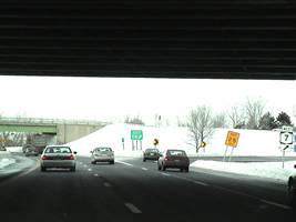
 [ Back ] [ Continue ] with Problem 3

Problem 3: Basic Freeway Sections

Figure 7 shows a view of Location E looking north. We took the picture at a spot that is about halfway through the weaving section at Location E. The sign to Route 7 west can be seen at the right-hand edge of the picture. The bridge immediately overhead is Route 7. The bridge in the background is the semi-direct ramp leading from Rte 7 westbound to I-787 southbound. The merge sign in the distance at the left-hand edge of the picture is associated with the location where the right-hand ramp from Rte 7 west merges with I-787 north.

Figure 8 shows a view looking east at Location L. The left-hand lane is the auxiliary lane that goes from Location F on the western end through to a point just beyond Location L. In fact, to the left in the picture you can see the place where the auxiliary lane rejoins Rte 7 east. The right-hand lane is simultaneously the end of the south-to-east loop ramp going from I-787 south to Rte 7 east and the beginning of the east-to-north loop ramp going from Rte 7 east to I-787 north. You can see the start of the east-to-north loop ramp in the right-hand side of the picture. In the distance, you can see the spot where the right-hand ramp from I-787 to Rte 7 joins Rte 7, which is also the start of the weaving section at Location B.

Figure 7. View of I-787 North at Location E just before the loop ramp diverges to go toward Route 7 west		Figure 8. View of Route 7 at Location L looking east

Might need a transition /closure paragraph that describes the sub-problems, how they’re organized, what they address, and which one comes next and why.

 [ Back ] [ Continue ] with Sub-problem 3a

Sub-problem 3a: Analysis of the North Section of Krome Avenue (Class I Two-lane Highway)

Step 1. Setup

In this sub-problem, we will replace the assumptions used in our planning analysis with field data. We will then be able to compare the HCM planning analysis from Problem 2 with the operations analysis presented in this problem.

Consider:

• What is the difference between the planning and operations analysis?

• What additional data that will be applied in the operations procedure?

Discussion:
Take a few minutes to consider these questions. Click continue when you are ready to proceed.

[ Back ] [ Continue ] with Sub-Problem 3a

Sub-problem 3a: Analysis of the North Section of Krome Avenue (Class I Two-lane Highway)

In sub-problem 2a, we produced an estimate of the LOS for the north section of Krome Avenue, assuming that it operates with the characteristics of typical two-lane highways of the same class. In this sub-problem, we will examine the assumptions and substitute observed values for this section to apply the more detailed operational procedures.

What is the difference between the planning and operations level analyses? It is important to recognize the difference between the planning and operational level procedures. The operational procedure estimates the level of service from computed performance measures that are compared against established LOS thresholds for those measures. The two performance measures are percent time spent following (PTSF) and average travel speed (ATS). The LOS thresholds for these measures are shown in Exhibit 3-17. For a Class I two-lane highway, the more critical of the two measures will determine the LOS.

The planning level procedure presented in HCM Chapter 12 was derived from the operational procedure, assuming typical values for all operating parameters. The service volume table in HCM Exhibit 12-15 was produced by applying the operational procedure repetitively with different volumes and noting the volume levels at which the LOS changed from one value to the next. As such, the service volume table results should be identical to the operational level results, but only when the same operating parameters are applied to both procedures.

For example, the service volume tables presented in the HCM and used within the planning analysis assumes 14% trucks and buses. Data collected for the Krome Avenue indicates the corresponding value for Krome Avenue is 27%. Similarly, the default peak hour factor for rural conditions assumed in the HCM is 0.88, whereas the actual measured PHF is 0.94. The differences between these values will cause the results of the two methods to depart from each other; and the operational level results must be considered more accurate, because they are based on actual field data instead of assumptions that do not apply to the facility under study.

[ Back ] [ Continue ] with Sub-Problem 3a

Sub-problem 3a: Analysis of the North Section of Krome Avenue (Class I Two-lane Highway)

The procedures given in HCM Chapter 20 will be applied to this section of Krome Avenue.

What is the additional data that will be applied in the operations procedure? The additional data (i.e., beyond the sub-problem 2a requirements) include:

• percent trucks

• directional distribution

• percent no passing zones

• shoulder width

• lane width

• PHF

• access points per mile

• segment length

The last item, segment length, is not actually required for estimation of LOS, but it is used for calculation of travel time and vehicle-miles of travel. All of these data items with their associated sources and assumptions were discussed in the Getting Started section of this case study.

[ Back ] [ Continue ] with Sub-Problem 3a

Sub-problem 3a: Analysis of the North Section of Krome Avenue (Class I Two-Lane Highway)

Step 2. Results

The table below compares the results from the planning level analysis in sub-problem 2a with the operational level analysis. This table shows the values assumed by the service volume tables for all parameters, as compared with the values that apply to this facility. It shows the computations and results for both methods. The ATS was computed as 45.2 mph, which suggests LOS C. The PTSF was computed as 66.9%, which suggests LOS D.

So, the resulting LOS was based on the PTSF and was found to be LOS D. This result was identical to the LOS estimate given by the service volume tables. The interpretation of the agreement between the two procedures is that the sum total of all of the differences between the assumed parameters and the site-specific parameters for this facility was not sufficient to produce a difference in the estimated level of service. 

[ Back ] [ Continue ] with Sub-Problem 3a

Sub-problem 3a: Analysis of the North Section of Krome Avenue (Class I Two-lane Highway)

The question of base free flow speed deserves further discussion. The service volume tables deal in 5 mph increments of free flow speed. The operational method requires a specified base free flow speed, which is adjusted to reflect the effects of the specified shoulder width and the number of access points per mile in computing the actual free flow speed. In the course of the computations, the actual free flow speed was adjusted downwards in this case by 1.5 mph. So, to promote a fair comparison, the base free flow speed was specified as 56.5 mph, to produce the same free flow speed of 55 mph that was used by the service volume tables. This modification to the base free would not normally be recommended as a sound analytical practice. It was applied in this sub-problem to facilitate comparison between the planning and operational level procedures.

The HCM Chapter 20 procedure has given an overall level of service for this facility based on the performance measures for two-lane roadways. This procedure does not recognize any intersection-related problems. Therefore, a complete assessment of the facility requires a check of all intersections to ensure that problems are not being overlooked. The proper procedures to apply to intersections are found in HCM Chapter 16 (signalized) and 17 (unsignalized). The details of the intersection analyses will not be presented here; however, it was found that two intersections experienced problems that will require further attention.

• The intersection with Okeechobee Rd operated under two-way stop control (TWSC). This is a T intersection in which Krome Avenue is stopped at its northern terminus. The northbound approach here is oversaturated, and mitigation measures will be required. The alternative measures will be discussed in Problem 4.

• The southern boundary of this section includes conditions that warrant further consideration. In this case, the cross street movements at Kendall Road are oversaturated. Mitigation measures will be discussed in Problem 5.

[ Back ] [ Continue ] to sub-problem 3b

Sub-problem 3a: Weaving Analysis

Another interesting observation occurs at Location B during the PM peak. The weave has a LOS B. Although the weave has adequate performance levels, a traffic signal located at the eastern end of Rte. 7 eastbound often creates long queues coming out of the weaving section. The queues are not caused by the weave, but do cause an impact in the way the weave operates.

Exhibit 2a-1. Weave C PM peak hour volumes

Weaving Segment C. The weave at location C is comprised of I-787 northbound, the 23^rd Street northbound on-ramp and the Rte. 7 eastbound off-ramp. This weave is a fairly conventional Type C weave. It has a length of approximately 1,000 ft. There is single lane on-ramp at 23^rd Street and a double lane off-ramp exiting to Rte. 7 eastbound.

We can use this weaving section to examine the effects that the flow distributions have on a weave’s performance. The PM peak hour volumes are heavier, so those will be used for the analysis. The PM peak hour volumes for traffic entering and exiting the weave are shown in Exhibit 1. The exhibit does not define the distribution of flows through the weaving segment. Let’s look at a three different scenarios.  

[ Back ] [ Continue ] with Sub-Problem 3a

Sub-problem 3a: Weaving Analysis

Figure 2. Scenario 1 weaving diagram

Figure 3. Scenario 2 weaving diagram

Figure 4. Scenario 3 weaving diagram

In the first scenario let’s see what happens if we assume that none of the traffic entering on the 23^rd Street on-ramp goes to Rte. 7 eastbound. In other words all of the Rte. 7 eastbound off-ramp traffic is associated with a weave from I-787 northbound. The weaving diagram for this scenario is shown in Figure 2.

In the second scenario, let’s see what happens if the percentages of the volumes going to C and D (from A and B) are proportional to the volumes exiting at C and D. Approximately 23% of the total exiting volume goes to Rte. 7 eastbound while 77% goes to I-787 northbound. Therefore in this case, the volume exiting at Rte. 7 eastbound would be comprised of: 23% of the entering I-787 northbound flow and 23% of 23^rd Street on-ramp flow. The weaving diagram for this scenario is shown in Figure 3.

In the third case let’s examine what happens if the percentage of vehicles entering at 23^rd Street and exiting at Rte. 7 eastbound is increased from 23% to 40%. The weaving diagram for this scenario is shown in Figure 4.

[ Back ] [ Continue ] with Sub-Problem 3a

Sub-problem 3a: Weaving Analysis

The results for these three performance analyses (Datasets XX, XX & XX) are shown in Table 2a-2. Due to the relatively low volumes, the LOS did not change greatly as we adjusted the distribution of the flows. This is important information. It means you don’t have to be extraordinarily worried about being precise about determining what the distributions are. It also means the facility’s performance is not that sensitive to what the distributions are. So if the distributions change from day to day or for other reasons, you’re assessment of the facility’s performance is still valid.

You should also realize that as the overall volumes in the weaving segment increase, these changes in the flow distributions will become more significant. If we focus on the changes in the densities, we can see that as the total number of weaving movements decreases the density decreases. You should also notice the impact that the distributions have on the various speed measures. As the weaving movements decrease and the non-weaving movements increase, both the weaving and non-weaving speeds both increase. This is to be expected because as the weaving volumes are reduced there is a decrease in the conflicts that arise in the segment allowing the speeds to increase. Therefore, the overall speed in the weave should also be expected to increase and the density should decrease.

Weaving Segment E. The weaving segment at location E is also interesting. It is a 3-lane, Type A weave located on I-787 northbound between an on-ramp (from Rte. 7 eastbound) and an off-ramp (to Rte.7 westbound). It is a short weave (792 feet) with heavy PM peak hour volumes. The weaving movements are easy to determine: very few if any of the people coming from the on-ramp want to go to the off-ramp. So, all of the on-ramp traffic goes north on 787 and all of the off-ramp traffic comes from 787 north. The free flow speed of the freeway is 55 mph, while the speed of the on- and off-ramps is 25 mph. The analyses will be done with a peak hour factor of 1.0.

[ Back ] [ Continue ] with Sub-Problem 3a

Sub-problem 3a: Weaving Analysis

This weaving section is a good place to examine the effects of varying the time period for the analysis. The PM peak hour volumes are more than twice the AM peak hour volumes (see Datasets XX & XX). The results of operational analyses for the AM and PM peaks are presented in Table 2a-3.

The operation of the weave during the AM peak is LOS B and during the PM peak it is LOS F. We should note that in these situations, the HCM suggests that the maximum volume ratio (VR) should be 0.45, and in both cases, this value is exceeded. This suggests that the segment may not be operating well, and some local queuing may be expected. The LOS F that is predicted in the PM peak analysis seems to match the performance observed in the field. During the PM peak, high volumes move through this short weaving section and often cause operational failure.

In order to consider the effect that peak hour factors and free flow speeds have on the weave performance, let’s perform a parametric analysis on the weave at Location E. For these analysis we will examine the PM peak hour and consider a variation of the peak hour factor from 0.8 to 1.0 with free flow speeds of 55 mph and 65 mph.

[ Back ] [ Continue ] with Sub-Problem 3a

Sub-problem 3a: Weaving Analysis

The results of these analyses are presented in Table 2a-4. Although the levels of service don’t indicate a significant effect, an examination of the densities and speeds measures more clearly demonstrates the impacts of PHF and free flow speed. The results clear show that as the peak hour factor increases the density of traffic in the weaving segment decreases and the speeds increase. The results also indicate that as the free flow speed is increased the densities decrease and the speeds increase. These trends are illustrated in Figure 5.  

[ Back ] [ Continue ] with Sub-Problem 3a

Sub-problem 3a: Weaving Analysis

Considering the poor operations at this facility it would be interesting to look at the effects that different geometric conditions would have on it operation. Let’s take the point of view, "we can start all over again". We’ll focus on two main ideas: increased length and additional lanes.

First, consider the question what effect does the weaving length have on the segments operations during the PM peak hour? The existing weave is 792ft in length. In order to observe the effects of the lengths, we’ll perform additional analyses for lengths of 1,000 ft to 2,500 ft. (Note 2,500ft is HCM’s the upper bound for the length of a weaving segment.) The results each of these analyses are shown in Table 2a-5. The results show that a minor increase in the weave length (approximately 200 ft) will bring the LOS from F to E. The second next step is quite a bit larger (around 1,500 ft); from LOS E to D.  

[ Back ] [ Continue ] with Sub-Problem 3a

Sub-problem 3a: Weaving Analysis

Let’s look at our second idea, the addition of a lane. Just upstream on I-787 northbound there is a two lane off-ramp, which effectively acts as a lane drop. Here we’ll examine the idea of maintaining that third lane through the weaving segment. The analysis results are presented in Table 6.

The impacts of the lane addition are significant. At the margin the LOS improves from F to D. The lane addition may also increase the free flow speed on the freeway (at location E) that would further improve the LOS to C.  

The weave at location E has shown the importance of considering multiple time periods, the effects of the free flow speed and peak hour factors, and the importance of geometric design in a weaving segment.

Weaving Segment D. The weaving movements at location D are far more complex. There is an upstream merge on the on-ramp and a lane drop in the middle of the weaving section. This weaving segment will be thoroughly examined in Sub-problem 2c.

Weaving Segment M. The weaving movements at Location M are also not traditional. The location a collector/distributor road located southerly of Route 7. There is single through lane with an additional lane between the I-787SB/Rte7EB on-ramp and the Rte7EB/I-787NB off-ramp. This section will be discussed in detail in sub-problem 2d.

[ Back ] [ Continue ] with Sub-Problem 3a

Sub-problem 3b: Operational Analysis of the Center Section of Krome Avenue (Class I or II Two-Lane Highway)

Step 1. Setup

In this sub-problem, we will replace the assumptions used in our planning analysis with field data for the center section of Krome Avenue. We will then be able to compare the HCM planning analysis to the operations analysis for this example, based on what is known about the assumptions made in the planning analysis verses the actual conditions along Krome Avenue.

Consider:

• What are the differences in analyses for Class I and II facilities?

• What LOS do you expect the results of the analysis to show?

Discussion:
Take a few minutes to consider these questions. Click continue when you are ready to proceed.

[ Back ] to Sub-Problem 3a [ Continue ] with Sub-Problem 3b

Sub-problem 3b: Operational Analysis of the Center Section of Krome Avenue (Class I or II Two-Lane Highway)

The procedures given in HCM Chapter 20 will be applied to this section. It was determined in sub-problem 1b that this facility has the characteristics that could normally be associated with both Class I and Class II two-lane highways. Therefore, the analysis will be repeated for both Class I and Class II facilities, and the results will be compared. The results will also be compared with those of the planning level analysis performed in sub-problem 2b.

What are the differences in analyses for Class I and II facilities? We will begin with a discussion of the differences in the LOS estimation procedures for Class I and II facilities.

As we pointed out in sub-problem 3a, the key performance measures for two-lane highways are the percent time spent following (PTSF) and the average travel speed (ATS). The LOS thresholds for these measures are shown in Exhibit 3-19 for both facility Classes.

On a Class I facility, the more critical of the two measures will determine the LOS. On a Class II facility, only the PTSF is considered, and the LOS thresholds for Class II are shifted upwards by 5 percentage points from Class I to reflect the lower driver expectation on a Class II highway. For example, the threshold for LOS E for Class I facilities is 80% and for Class II facilities it is 85%. One important point is that the performance measures will be computed in exactly the same way for both Classes. In other words, the Class that you specify will not affect either the PTSF or the ATS. Only the thresholds will be applied differently.

[ Back ] [ Continue ] with Sub-Problem 3b

Sub-problem 3b: Operational Analysis of the Center Section of Krome Avenue (Class I or II Two-Lane Highway)

What LOS do you expect the results of the analysis to show? This is difficult to determine because of the differences in the criteria used between the two class types. As we will see in the next few pages, the various criteria lead to different estimates for LOS.

Which factor do you expect to determine the level of service on a Class I Facility? In a vast majority of cases involving Class I two-lane roadways, the LOS will be determined by the PTSF. On the rare occasion that the ATS emerges as the determining factor, it is a good idea to revisit the question of whether this really should be considered as a Class I facility. The ATS will generally be the critical determinant of LOS only when the free flow speed is low. A low free flow speed is frequently the result of the same factors that would reduce the driver’s expectation of a high speed. As a Class I facility, the operation of this section of Krome Avenue would probably be considered unacceptable at LOS E. As a Class II facility it would fall into LOS D, only 1/10 of a PTSF percentage point away from LOS C (70.0% vs 70.1%). This raises a separate but frequently stated point about the value of judgment in dealing with thresholds.

[ Back ] [ Continue ] with Sub-Problem 3b

Sub-problem 3b: Operational Analysis of the Center Section of Krome Avenue (Class I or II Two-Lane Highway)

Step 2. Results

Exhibit 3-20 compares the results from the planning level analysis in sub-problem 2b with the operational level analysis. It shows the values assumed by the service volume tables for all parameters, as compared with the values that apply to this facility. It also shows the computations and results for both methods. The ATS was computed as 39.3 mph. The PTSF was computed as 70.1%.

If this facility were designated as a Class I highway, the ATS would be the critical determinant of LOS, producing a value of E. The PTSF would have suggested LOS D. If the designation were changed to Class II, the ATS would be eliminated as a determinant of LOS, and the PTSF would establish LOS D.

[ Back ] [ Continue ] to Sub-Problem 3c

Sub-problem 3b: Operational Analysis of the Center Section of Krome Avenue (Class I or II Two-Lane Highway)

The decision on class designation rests solely with the operating agency. The purpose of this guide is to point out the factors that should be taken into consideration and their relationship to the HCM procedures. Therefore, the question of whether this portion of Krome Avenue should be a Class I or II facility will remain open.

Before we leave this sub-problem, we should take a look at how the operational analysis results compared with the service volume table results from sub-problem 2b. The comparison is evident in the table on the next page. The bottom line is that, for a Class I facility the same estimation of LOS was produced by both procedures. While the LOS was improved for a Class II facility for the reasons just stated, it is not possible to compare this result with the service volume tables, because those tables are limited in scope to Class I facilities.

One last point: the base free flow speed was adjusted upwards to produce the same actual free flow speed used in the service volume tables to facilitate the comparison of the planning and operational level analyses. This topic was explained in detail in sub-problem 3a. The amount of the adjustment in this case was 3.1 mph, resulting in a base free flow speed of 53.1 mph in the table below.

[ Back ] [ Continue ] with Sub-Problem 3b

Sub-problem 3b: Operational Analysis of the Center Section of Krome Avenue (Class I or II Two-Lane Highway)

The HCM Chapter 20 procedure has given an overall level of service for this facility, based on the performance measures for two-lane roadways. This procedure does not recognize any intersection-related problems. Therefore, a complete assessment of the facility requires a check of all intersections to ensure that problems are not being overlooked. The proper procedures to apply to intersections are found in HCM Chapter 16 (signalized) and 17 (unsignalized). The details of the intersection analyses will not be presented here.

Apart from the northern boundary at Kendall, which was mentioned in sub-problem 3a, the only operational problem was found at Howard. This is an unsignalized intersection with the cross street operating under stop control. Signalization will be required to overcome this deficiency. The signalized intersection analysis will not be covered in this case study.

[ Back ] [ Continue ] with Sub-Problem 3b