Problem 1: U.S. 95/Styner-Lauder Avenue Intersection We will begin our work by considering the operations of the intersection of U.S. 95/Styner-Lauder Avenue under two kinds of control, the existing stop-sign control and the proposed signal control. In problem 1, we will focus our attention only on this intersection, without consideration of the effects of the adjacent intersections. This approach will allow us to develop an initial assessment of whether stop-sign control is better than signalized control, but we must keep in mind that other factors (including, for example, the proximity of adjacent intersections and the manner in which they are controlled) can also have a very big influence on our final recommendation. These effects will be considered later in Problem 2. For this particular analysis, we must first complete two computations for the existing traffic volume conditions. Then, we will consider the projected future volumes. We can pose three questions that will guide the computations:
Discussion: |
Page Break
Problem 1: U.S. 95/Styner-Lauder Avenue Intersection In this problem, you will consider the following issues as you work through the computations for three sub-problems: Sub-problem 1a: Analysis of
the existing TWSC intersection Sub-problem 1b: Analysis of
the proposed signalized intersection Sub-problem
1c: Analysis of future conditions |
Page Break
Sub-problem 1a: Analysis of the existing TWSC intersection Step 1. Setup The analysis of transportation facilities can be complex, requiring both the skilled use of standard computational procedures such as the HCM as well as good judgment in the use and interpretation of results from the computational procedures. In the setup of this problem, we will consider the data, the issues, and the tools that are relevant to this problem. In particular, we will consider the analysis of the U.S. 95/Styner-Lauder Avenue intersection under two-way stop-control. Here are some issues to consider as you proceed with the analysis of the existing intersection and its performance:
Discussion: |
Page Break
Sub-problem 1a: Analysis of the existing TWSC intersection Let's discuss each of these issues and how each affects the operational analysis that we are about to complete. Which tool or tools from the HCM should be used for this analysis? The analysis tools for unsignalized intersections are contained in chapter 17 of the HCM 2000. Chapter 17 includes analysis tools for two-way stop-controlled (TWSC) intersections, all-way stop-controlled (AWSC) intersections, and roundabouts. In this analysis, we will use the procedure for TWSC intersections. Since we are interested in existing conditions at the intersection, at a fairly detailed level, we will use the operational analysis procedure in chapter 17. What data are required for the analysis? Since we are interested in determining the average control delay that drivers experience at the existing intersection, we will use the operational analysis method that is included in chapter 17 of the HCM. The following data are needed to conduct an operational analysis:
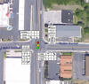
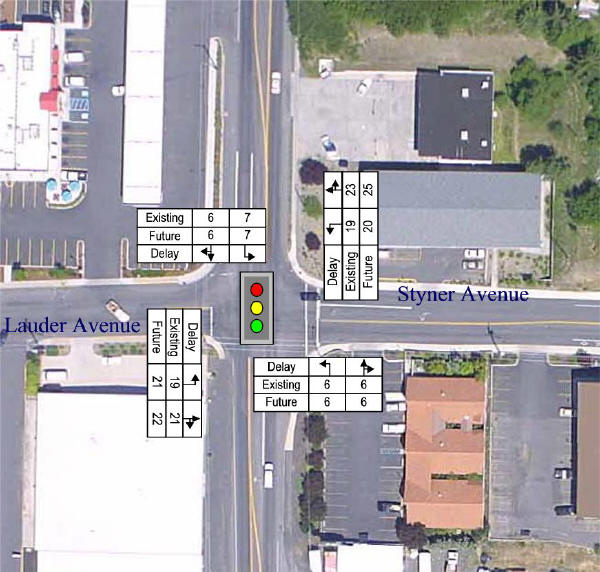
We should note one potential point of confusion in the aerial photograph for this intersection. While the eastbound approach striping does not show this explicitly, this approach does operate as if it is configured with an exclusive left turn lane and a shared through/right turn lane. These details are always important to check in the field. |
Page Break
|
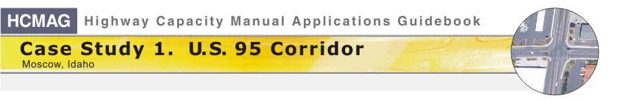
Exhibit 1-6. Aerial Photograph of the Intersection of U.S. 95 with Styner Ave/Lauder Ave The intersection of U.S. 95/Styner Avenue/Lauder Avenue is a four leg TWSC intersection. The westbound approach, Styner Avenue, serves a growing residential area in the eastern section of the city. Lauder Avenue serves as a minor entrance to the University of Idaho and access to student and faculty residences. A gas station/mini-mart is located on the northwest quadrant of the intersection. Other auto-oriented businesses are located on the other quadrants. Note: You can see other views of the intersection approach by moving your mouse to the approach and clicking on the approach.
|
Page Break
Sub-problem 1a: Analysis of the existing TWSC intersection Following are other points to consider regarding the required data:
|
Page Break
Sub-problem 1a: Analysis of the existing TWSC intersection What default values should be used? Driver behavior at a TWSC intersection is described by two parameters, the critical gap and the follow up time. The HCM provides default values that represent average values from a number of measurements made at sites throughout the United States for critical gap and follow up time. However, conditions at the site (unusual geometric features, high volumes causing more aggressive driver behavior) that you are studying may produce values that are different than these default values. It is always better to use values that are estimated from the site that you are studying, if these values can be measured. However, it should be pointed out that critical gaps cannot be directly measured in the field. Rather, they are estimated using statistical procedures based on the distribution of gaps that are accepted and rejected by drivers in the field. An appropriate but somewhat complex method for doing this was presented by Troutbeck in 1992. A rough method to check the validity of the critical gap would be to measure the follow-up time, which can be done easily, and to estimate the critical gap using the approximate relationship, tf/0.6. What time periods should be analyzed? The data that have been collected for this site represent the volumes for the afternoon peak period. If there are other peak times during the day, such as the morning peak or sometimes a midday peak, these should also be included in an operational analysis. What measure should be used to determine the performance of the intersection? The level of service for a TWSC intersection is based on control delay. Control delay is the primary measure of effectiveness for TWSC intersections and will be used as the parameter to compare the performances of the various alternatives that we consider in this problem. In fact, control delay is also used as the primary measure of effectiveness for signalized intersections. In addition, we will consider two other performance measures, each describing another aspect of the operation of the intersection. The v/c, or volume/capacity ratio is useful for showing how close the intersection is to capacity operation. The queue length provides a way for the analyst to determine the adequacy of the geometric design of the facility by examining the projected length of a queue compared with the length of turning or storage lanes. |
Page Break
Sub-problem 1a: Analysis of the existing TWSC intersection What other factors should be considered? One of the important elements in determining the capacity of each minor movement at a TWSC intersection is the conflicting flow, which is defined as that flow to which the minor movement must yield the right of way. For this problem, we might pay particular attention to the northbound right turn movement. If you study the aerial photograph for this approach (link), you will note that there is a flare, providing a short lane for right turning vehicles. We should also study whether or not right turning vehicles commonly used this lane, and, if so, whether this results in a lower conflicting flow faced by the minor street movement. At first glance, you might conclude that the right-turning traffic shouldn't even be included as one of the conflicting traffic streams since there is no physical conflict with any of the minor movements. However, field studies have shown that minor street drivers are reluctant to initiate their movement until they can be sure that the approaching vehicle is in fact going to make a right turn. It is for this reason that the HCM includes the major street right-turn volume as a potential conflict; the 0.5 factor associated in some instances with this right-turn volume was determined through field studies to be an appropriate "calibration factor" that accounts for the hesitancy minor street drivers often exhibit when confronted with an apparent right-turning vehicle. It should be noted that the HCM suggests that the major street right turn movement from a separate lane be entirely excluded from the conflicting flows for the minor street movement because, in such cases, the minor street drivers are usually quite confident that the approaching vehicle is actually going to make a right turn. In the case of this particular sub-problem, the flare or right-turn lane is very short, and so we will assume that the effect of the right turning vehicles is accounted for with the 0.5 factor assumed in the HCM procedure. For a complete discussion of the conflicting flow rates, see Exhibit 17-4 of the HCM. Review the traffic data to see the existing afternoon peak period volumes for this site. |
Page Break
Sub-problem 1a: Analysis of the existing TWSC intersection Step 2. Results The HCM capacity analysis procedure for TWSC intersections produces the following results for each minor stream movement:
For the input data that we are considering here, the results are summarized in Exhibit 1-9.
The table shown above provides a substantial amount of information regarding the forecasted operation of the intersection, including the estimated capacity, v/c ratio, queue length, and delay. What information from the table is most relevant to our analysis? Discussion: |
||||||||||||||||||||||||||||||||||||||||||||||||||||||||||||||||||||||||||||||||||||||||||||||||||||||||||||||||||||||
Page Break
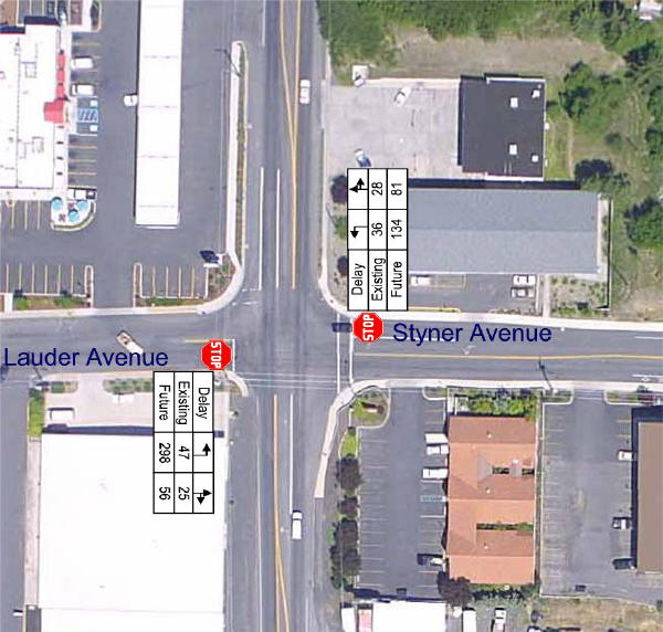
Sub-problem 1a: Analysis of the existing TWSC intersection Level of service (LOS) for a TWSC intersection is determined by the control delay and is defined for each movement, but LOS alone does not tell the whole story! Besides LOS, other performance measures that should also be considered include the volume/capacity ratios and the estimated queue length. Let's investigate each of these measures of effectiveness in greater detail (see Exhibit 1-9). First, note that the left turn movements on the major street (NBLT and SBLT, movements 1 and 4), experience acceptable delay. The HCM methodology estimates that both movements will experience level of service A, with less than 10 seconds of control delay per vehicle. We can also see that the movements on the minor street approaches (westbound on Styner and eastbound on Lauder) experience moderate to high levels of delay. Both left turn movements (movements 7 and 10), for example, operate at level of service E with delays of 36 and 47 seconds, respectively. The volume/capacity ratio is also important to consider because it tells us how close we are to capacity for each movement. Here, the v/c ratio is less than 0.60 for all movements. Thus, there is ample capacity available for the existing conditions. Queue length is always an important consideration at an unsignalized intersection, and especially when it is necessary to determine the adequacy of turning bays or when there is the possibility of a queue spilling back into the adjacent upstream intersection. In the case of the Styner-Lauder/U.S. 95 intersection, the 95th-percentile queue length estimates are less than four vehicles, meaning that there is sufficient space to store vehicles as they are waiting to enter the intersection. Even so, the queue length requirements for the right turns from the minor street (movements 9 and 12) are 3 vehicles. This is a length that some drivers might consider to be excessive (even though it only has a 5 percent probability of occurring), and especially so for drivers in a smaller community like Moscow. |
Page Break
Sub-problem 1a: Analysis of the existing TWSC intersection Note in the Exhibit 1-9 how delay and level of service are reported. First, the results are reported for each movement. Then, the results for the minor street approaches are reported. What is the value in showing both results? The results for each movement allow the analyst to see the operation of the intersection at the smallest level. If any one movement is experiencing a high delay, such as movement 10, attention can be paid to resolving that problem. The approach data provides a broader look at the intersection performance and is often useful when comparing the operation of a number of intersections. Finally, you should note that the delay and level of service for the entire intersection is not reported. This is in part due to the assumed zero delay for the major street through and right turn movements and the importance of monitoring the operation of the minor street movements. In any case, it is important to remember that, for an unsignalized intersection as a whole, LOS is undefined. In summary, a review of the performance characteristics indicates that the intersection is operating acceptably, but in a marginal range with respect to both control delay and queue lengths. Now that we've completed the analysis of the existing TWSC intersection, we'll proceed to the analysis of the intersection under the proposed signal control.
|
Page Break
|
|
|
Exhibit 1-9. U.S. 95/Styner Avenue-Lauder
Avenue
(Dataset1) |
||||||||
|
Approach |
NB |
SB |
Westbound |
Eastbound |
||||
|
1 |
4 |
7 |
8 |
9 |
10 |
11 |
12 |
|
|
L |
L |
L |
|
TR |
L |
|
TR |
|
|
31 |
59 |
55 |
|
205 |
50 |
|
155 |
|
|
1,024 |
1,163 |
170 |
|
359 |
134 |
|
329 |
|
|
0.03 |
0.05 |
0.32 |
|
0.57 |
0.37 |
|
0.47 |
|
|
95% queue length (vehicles) |
0.09 |
0.16 |
1.31 |
|
3.39 |
1.56 |
|
2.41 |
|
Control delay (sec/veh) |
8.6 |
8.3 |
36.0 |
|
27.6 |
47.0 |
|
25.3 |
|
LOS |
A |
A |
E |
|
D |
E |
|
D |
|
Approach delay (sec/veh) |
-- |
-- |
29.3 |
30.6 |
||||
|
Approach LOS |
-- |
-- |
D |
D |
||||
Page Break
Sub-problem 1b: Analysis of the Proposed Signalized Intersection Step 1. Setup We will now consider the operation of the U.S. 95/Styner-Lauder intersection under signal control. Here are some issues to consider as you proceed with this analysis of the existing intersection.
Discussion: |
Page Break
Sub-problem 1b: Analysis of the Proposed Signalized Intersection Let's discuss each of these issues and how each affects the operational analysis that we are about to complete. Which tool or tools should be used for this analysis? There are a number of tools that the analyst might consider to solve this problem. A hand-calculated critical movement analysis or the HCM planning analysis might be considered to get a quick assessment of the intersection performance and operation. These are both discussed at greater length in Problem 6 in this case study. Other non-HCM tools such as Synchro, CORSIM, or aaSIDRA might be used. Finally, the HCM operational analysis method for signalized intersections, which produces estimates of control delay, v/c ratio, and queue length, is a potential tool for this sub-problem. We will use this latter tool for this analysis. Why did we make this choice? When we are considering conditions in which demand does not exceed capacity, or the flows from one intersection do not spill back and affect the adjacent upstream intersection, the HCM operational analysis method provides a useful and easily applied tool. In addition, we are conducting a comparative analysis between signalized and unsignalized intersection operational characteristics, so we are looking for procedures that allow this kind of comparison to be made easily and consistently. We will explore the use of non-HCM tools in problems 3 and 4 of this case study. We will address some of the major issues that are often confronted by analysts using the HCM methodology in this and subsequent problems in this case study. The analysis tools for signalized intersections are contained in chapter 16 of the HCM 2000. The computational methodologies included in this chapter are complex and cover a wide range of conditions that are often observed in the field. |
Page Break
Sub-problem 1b: Analysis of the Proposed Signalized Intersection What data are required for the analysis? The following data are needed to conduct an operational analysis:
What default values should be used? There are a number of traffic and geometric conditions for which default values have been established. Each condition must be considered and a decision made regarding whether field data should be used to override these default values:
|
Page Break
Sub-problem 1b: Analysis of the Proposed Signalized Intersection What time periods should be analyzed? The data that have been collected for this site represent the peak 15-minute flow rates for the afternoon peak period. A 15-minute analysis is used here (as opposed to the one-hour analysis used for the existing stop sign control described in sub-problem 1a) because signalization is an expensive mitigation option that almost always adds to total system delay. Therefore, we want to evaluate it at a higher standard -- that is, we want to be sure it is able to perform adequately even during the peak 15 minutes of the peak hour. If there are other peak times during the day, such as the morning peak or sometimes a midday peak, these should also be included in an operational analysis. Since we are considering a decision that may take several years to implement, we will also consider traffic conditions that are expected over the next ten years. Review the traffic data to see the existing and projected afternoon peak period volumes for this site. This is also discussed in Problem 3 when we consider an analysis of event traffic following a football game. How do we construct a signal timing plan for a proposed traffic signal using the HCM? The construction of a timing plan for a signalized intersection can be a complex process, though there are also some simple approaches that give very reasonable first-approximations. In this problem, we will assume that the proposed new signal will operate in fixed time mode, and the methods included in Appendix B of Chapter 16 of the HCM can be used to determine the signal timing plan for this condition. There are other tools that can be used for developing signal phasing and timing plans including the Institute of Transportation Engineers (ITE) Traffic Engineering Handbook, as well as the ITE guidelines for left turn phasing. The critical movement analysis technique is another good way to quickly develop a reasonable signal phasing and timing plan. The decision to signalize the intersection or not does not depend on whether the traffic controller is fixed time or actuated. To simplify this analysis, then, we have chosen to assume that it will operate in fixed time mode. In Problem 4, we will illustrate how the HCM procedure considers actuated controller operational parameters. The following signal timing was produced for this sub-problem, using the methods of Appendix B, chapter 16, of the HCM.
Click continue below to proceed with the analysis. |
||||||||||||||||||||||
Page Break
Sub-problem 1b: Analysis of the Proposed Signalized Intersection Step 2. Results When we apply the methods of chapter 16 of the HCM, we obtain estimates of capacity, v/c ratio, queue length, delay, and level of service for each lane group. In addition, capacity, delay, and level of service are produced for each approach. Also, the delay and level of service are produced for the intersection as a whole. The results from this calculation are summarized in Exhibit 1-11 for the existing volumes and signalized intersection control.
Discussion: |
|||||||||||||||||||||||||||||||||||||||||||||||||||||||||||||||||||||||||||||||||||||||||||||||||||||||||||||||||||||||||||||||
Page Break
Sub-problem 1b: Analysis of the Proposed Signalized Intersection A review of the information contained in Exhibit 1-11 provides the following insights on the current operation of this intersection, if it were to be controlled by a traffic signal:
It is important to consider each of these three levels of analysis (intersection as a whole, approach, and lane group). Each level tells the analyst something different, and important, about the operation of the intersection. Intersection level of service is important when comparing a number of design alternatives or when comparing a number of different intersections in a study area. Approach and lane group level of service is important when identifying operational problems with specific traffic movements or signal timing allocation among phases. In problem 4, we will consider various signal operations strategies and their implications on the measures of effectiveness (MOEs) at the intersection. |
Page Break
|
Exhibit 1-11. U.S. 95/Styner-Lauder Avenue (Dataset2) |
||||||||
| EB | WB | NB | SB | |||||
| LT | TH/RT | LT | TH/RT | LT | TH/RT | LT | TH/RT | |
| Adjusted flow rate | 50 | 155 | 55 | 205 | 31 | 407 | 59 | 557 |
| Lane group capacity | 276 | 438 | 313 | 432 | 491 | 2,067 | 569 | 2,012 |
| v/c ratio | 0.18 | 0.35 | 0.18 | 0.47 | 0.06 | 0.20 | 0.10 | 0.28 |
| 95% queue length | 1.6 | 4.8 | 1.8 | 6.3 | 0.6 | 3.9 | 1.1 | 5.4 |
| Green ratio | 0.25 | 0.25 | 0.25 | 0.25 | 0.58 | 0.58 | 0.58 | 0.58 |
| Control delay | 19.0 | 20.7 | 18.9 | 22.9 | 5.7 | 6.1 | 5.9 | 6.6 |
| Lane group LOS | B | C | B | C | A | A | A | A |
| Approach delay | 20.3 | 22.0 | 6.1 | 6.5 | ||||
| Approach LOS | C | C | A | A | ||||
| Intersection delay | 10.9 | Intersection LOS | B | |||||
| Critical v/c ratio | 0.34 | |||||||
Page Break
Sub-problem 1c: Analysis of Future Conditions Step 1. Setup In addition to assessing the performance of the intersection with existing traffic conditions as we did in sub-problems 1a and 1b, we also need to look to the future to determine what conditions will be like at some future time. Any significant transportation investment, such as the installation of a new traffic signal, must be considered over time, not just with the existing conditions. For that reason, we will now analyze the performance of the intersection of U.S. 95/Styner-Lauder, under both control conditions, using future traffic volumes. Here are some issues to consider as you proceed with the analysis of both TWSC and signal control, assuming future traffic volumes.
Discussion: |
Page Break
Sub-problem 1c: Analysis of Future Conditions Let's consider the answers to these questions. What is the appropriate future year for this analysis? The appropriate horizon for a future year analysis depends on a number of factors. Often, an agency has a standard target year (based on a regional travel demand model) on the order of five, ten, or twenty years. Sometimes the horizon is selected based on the level and type of the investment under consideration. For a major freeway investment, twenty years is often used. For a new signal installation, ten years is often used. We will use a ten year horizon for this analysis. Which default values should be used for this future analysis? While we can take field measurements to determine the appropriate input data and default values to use for the analysis of existing conditions, this is not possible for a future analysis. What we must do is to use the existing data as a guideline and then, based on what we know about the projected changes in traffic conditions and in the transportation system itself, make estimates of these future values. For the analysis of future conditions at the intersection, we must also consider how to establish reasonable values for other critical analysis parameters. For an unsignalized intersection analysis, the additional critical parameters include peak hour factor, critical gap, follow up time, and heavy vehicle percentage. For a signalized intersection analysis, these critical parameters include arrival type, saturation flow rate, peak hour factor, and heavy vehicle percentage. |
Page Break
Sub-problem 1c: Analysis of Future Conditions Step 2. Results For the analysis of future conditions, it is often appropriate to select a peak hour factor of 1.0, considering that the projected future volumes, as well as other critical analysis parameters, have a relatively high degree of uncertainty associated with them. In this context, then, using a peak hour factor of 1.0 is equivalent to evaluating the intersection on the basis of the estimated average conditions for the hour rather than the peak 15 minutes. In many cases, the accuracy resulting from this approach is on par with the cumulative accuracy that one can expect for the other critical analysis parameters that must also be estimated. The value of the arrival type for the signalized intersection option depends on whether the signal will be interconnected with the adjacent intersections and the quality of progression that will be achieved. It is usually conservative to assume random arrivals (Arrival Type 3). The values of the saturation flow rate, the critical gap, and the follow up time depend on local conditions and whether, as volumes increase, driver behavior may change over time. We will assume for this analysis that they remain the same as the original analysis. These are all reasonable assumptions, but most likely the assumptions are less accurate than the estimates we were able to prepare for the existing conditions analysis. What other factors should be considered? In addition to the factors discussed above, we must also have forecasts of future volume levels. In order that they might be as accurate as possible, future volume projections should not just consider historic patterns of growth but also current local policies regarding development. For example, if growth management policies are in effect, future growth may be lower than historical patterns. And, since we can't know precisely the composition of the traffic stream with respect to vehicle types, it is again usually conservative to assume a passenger car equivalence of 1.1. For this case study, we are unaware of any land use policies that might change historic growth trends. Since we know that traffic volumes on U.S. 95 are increasing at the rate of 2 percent per year, it is conservative to assume that this rate will continue and that, with compounding, the volumes in ten years will be about 22 percent higher than today's volumes. Click here to see the future traffic volumes. Let's continue to see the results of the computation. |
Page Break
Sub-problem 1c: Analysis of Future Conditions The results of the HCM analysis for the two types of
intersection control under future traffic flow conditions for the intersection of
U.S.
95/Styner-Lauder Avenue are shown in the following tables.
Discussion: |
|||||||||||||||||||||||||||||||||||||||||||||||||||||||||||||||||||||||||||||||||||||||||||||||||||||||||||||||||||||||||||||||||||||||||||||||||||||||||||||||||||||||||||||||||||||||||||||||||||||||||||||
Page Break
Sub-problem 1c: Analysis of Future Conditions For TWSC (see Exhibit 1-12):
|
Page Break
Sub-problem 1c: Analysis of Future Conditions For signal control (see Exhibit 1-13):
Discussion: |
Page Break
Sub-problem 1c: Analysis of Future Conditions Uncertainty analysis is often used to consider the effects that uncertainty in the input values for a problem will have on the outputs, and whether these effects will be significant. To illustrate this kind of analysis, we will consider three cases. The first case is the base case, where we assume that the volumes that we used are correct. The second case assumes that our volume forecasts are high by 25 percent, while the third case assumes that the volume forecasts are low by 25 percent. Exhibit 1-14 focuses exclusively on a single performance measure (average control delay), though in reality we would also want to explore the impact on other performance measures such as v/c ratio and queue length.
Exhibit 1-14 shows two very interesting points. First, for the minor movements at the TWSC intersection, the volume changes have a large impact on the final results. This shows that the projected operation of the intersection is unstable to begin with, and that any increase in the volumes will further degrade the intersection performance. Second, we can have some degree of confidence that, under signal control, the intersection will perform as planned, even if we are somewhat uncertain about the input volumes that we've projected. These results can help decision-makers feel more certain about the range of possible ramifications associated with different control decisions. In addition to varying the input volumes, we could also determine the sensitivity of other input or default values on the final results. For example, the critical gap, the follow up time, the saturation flow rate, and the arrival type are all important parameters in the computation of capacity and delay. The base case values for these parameters could also be varied to determine their effect on the final results. |
||||||||||||||||||||||||||||||||||||||||||||||||||||||||||||||||||||||||||||||
Page Break
Sub-problem 1c: Analysis of Future Conditions Exhibit 1-15 and Exhibit 1-16 below shows the average control delay per vehicle for the minor street approaches (Lauder Avenue and Styner Avenue) for both the existing and projected traffic volumes under both TWSC and signal control. Preparing graphic representations of delay often helps you to better visualize the relative performance of the various movements at an intersection. Another view of this data is shown on the next page. |

Page Break
|
TWSC Intersection - Existing and Future Delay Estimates
|
Page Break
|
Signalized Intersection - Existing and Future Delay Estimates
|
Page Break
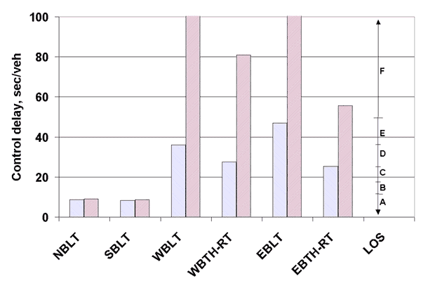
Sub-problem 1c: Analysis of Future Conditions Exhibit 1-17 shows a plot of the delay and level of service for each minor stream movement for both the existing conditions and projected ten year conditions, under TWSC. The existing conditions are shown in blue on the left, while the projected conditions are shown in red on the right. Each of the movements on the minor streets (Styner and Lauder) degrade to LOS F in ten years. This performance is below standards established by both the City and the Idaho Transportation Department, and clearly show that consideration should be given to changes in either the intersection geometry or control. How can we integrate the information from the analyses of both intersection control options in a way that is useful to a decision maker? |
Page Break
|
U.S. 95/Styner-Lauder Avenue TWSC Intersection - Existing and Future Conditions
|
Page Break
Problem 1: Analysis of the U.S. 95/Styner-Lauder Avenue Intersection We will now integrate the results from the three computations, considering the intersection U.S. 95/Styner/Lauder under TWSC and signal control. Let's begin with a comparison of the overall delay experienced by all drivers who would use the intersection. This intersection delay is calculated explicitly as part of the HCM method for signalized intersections. For the TWSC intersection, we will assume that the delay is zero for major street through and right turn vehicles and compute a weighted average of delay for all vehicles entering the intersection. But while we can compute the average intersection delay for a TWSC intersection, we should note that the HCM explicitly does not define level of service for the intersection as a whole. This fact should encourage the user to look carefully at the operation of each minor movement. We should also be reminded that both v/c ratio and queue length should be considered when reviewing the overall performance of the TWSC intersection.
When a signal is added, the delay is shifted from some movements to other movements. In this case, the northbound and southbound traffic on U.S. 95 experience no delay when the side streets (the eastbound and westbound movements) are stop sign controlled. But when a signal is added, these movements will also experience some delay. In fact, the average delay for all vehicles increases by a small amount when the intersection control is changed from TWSC to signal control. The benefits of the signalized control, however, are shown when the future conditions are considered. The additional delay for all vehicles increases by a small amount, while for TWSC the delay increases significantly from about 10 seconds per vehicle to about 32 seconds per vehicle. This difference is more dramatic when considering individual movements or lane groups. For example, for existing volumes, the WB LT movement would experience almost a 50 percent decrease in delay (from 36 seconds to about 19 seconds) if the intersection were signalized. with Analysis |
||||||||||||||||
Page Break
Problem 1: Analysis of the U.S. 95/Styner-Lauder Avenue Intersection
A review of the information contained in Exhibit 1-19 provides important information to think about as the decision to signalize the intersection (or not) is considered:
The information presented here indicates that changing from TWSC to signal control will improve the operation of this intersection, particularly over the next ten years. The uncertainty analysis that we conducted as part of sub-problem 1c confirms that this decision is a sound one.Discussion: to Problem 1 Discussion |
||||||||||||||||||||||||||||||||||||||||||||||||||||||||||||||||
Page Break
Problem 1: Discussion of the U.S. 95/Styner-Lauder Avenue Intersection The analysis presented thus far using the HCM methodologies for Chapters 16 and 17, and the conclusions reached using these methodologies, all seem relatively straightforward. The delay for the minor movements at the TWSC intersection of U.S. 95/Styner-Lauder Avenue will continue to increase during the next ten years. Installing a signal at the intersection, while somewhat inconveniencing traffic on U.S. 95 that currently operates with no delay, will improve traffic operations. But have we taken a thorough look at the situation, or is there more to consider? Yes, there is more to this story! We considered the U.S. 95/Styner-Lauder Avenue intersection as isolated in our initial analysis, but in reality, most intersections do not operate in isolation, and the U.S. 95/Styner-Lauder Avenue intersection is no exception. Let's consider what kind of a system this intersection is a part of. Review the sketch and aerial photograph to remind yourself of the geometric layout of the U.S. 95 corridor.
If we consider the U.S. 95/Styner-Lauder Avenue intersection to be a part of this arterial system, there are several new issues that must be considered in our analysis:
Discussion: |