Problem 1: Maxwell Drive The intersection of Maxwell Drive with Route 146 (Intersection C) is signalized and fully actuated. About 2,000 feet to the east is the intersection of Clifton Country Road and Route 146 (Intersection D), 4,000 feet to the west is the intersection of Moe Road and Route 146 (Intersection B), and 300 feet to the north is the Intersection of Park Avenue and Maxwell Drive. All three of these upstream intersections are signalized and fully actuated.
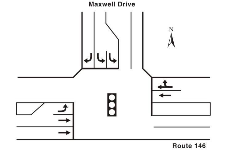
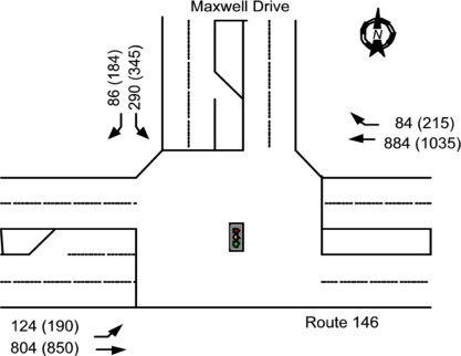
As Exhibit 2-4 shows, the eastbound approach of the Maxwell Drive/Route 146 intersection is three lanes wide (left, and a double through) while the westbound approach is two lanes wide (through and through/right). The eastbound left-turn bay is approximately 100 feet, while the southbound left-turn bay is approximately 125 feet. The approach for Maxwell Drive itself (the southbound approach) is three lanes wide (double left and right). Base Case Phasing and Volumes Analysis Plans Description of Analyses Sub-problem 1a: PM Peak Hour - Existing Conditions
Sub-problem 1b: Discussion:
|
Page Break
Problem 1: Maxwell Drive Base Case Phasing
Base Case Volumes
Exhibit 2-6
|
||||||
|
to Analysis Plans |
Page Break
|
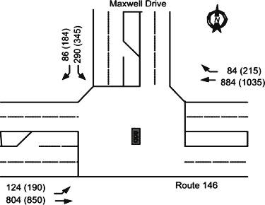
Exhibit 2-6. Maxwell Drive Intersection Volumes for the Existing AM & (PM) Peak Hour
|
Page Break
Sub-problem 1a: Maxwell Drive PM Peak Hour - Existing Conditions The intersecting volumes by 15-minute intervals for the existing PM Peak are shown in Exhibit 2-7. You can also see that the peak hour is from 17:00-18:00. The total number of intersecting vehicles is 2,877 and the overall peak hour factor (PHF) is 0.94. The movement-specific peak hour factors range from 0.78 to 0.95, with those for the major movements being fairly high and consistent, while those for the the minor movements are lower and more variable. Moreover, the minor movements seem to offset each other in terms of contributing to the 15-minute volumes.
For the purposes of this problem, we will apply the overall PHF of 0.94. It is, of course, also possible to apply each of the peak hour factors for the individual movements as discussed above, but doing so would presume that all of the individual movements peak during the same 15-minute time period of the hour. This does not happen very often, and so application of the overall PHF normally results in a more realistic assessment of intersection operations during the peak 15-minute period. Analyses: Discussion:with Sub-problem 1a |
|||||||||||||||||||||||||||||||||||||||||||||||||||||||||||||||||||||||||||||||||||||||||||||||||||||||||||||||||||||||||||||||||||||||||||||||
Page Break
Sub-problem 1a: Maxwell Drive PM Peak Hour - Existing Conditions Base Case Analysis Exhibit 2-8 presents the base case results for signal timings that about equalize the delays for the critical movements in each phase. The movement-specific delays range from 5.3 to 20.8 seconds per vehicle and the average queue lengths range from 1.8 to 9.9 vehicles.
with Sub-problem 1a |
||||||||||||||||||||||||||||||||||||||||||||||||||||||||||||||||||||||||||||||||||
Page Break
Sub-problem 1a: Maxwell Drive PM Peak Hour - Existing Conditions Arrival Type
Changes
Discussion: to Sub-problem 1a |
||||||||||||||||||||||||||||||||||||||||||||||||||||||||||||||||||||||||||||||||||||||||||||||||||||||||||||||||||||||||||||||||||||||||||||||||||||||||||||||||||||||||||||||||||||||||
Page Break
Sub-problem 1a: Maxwell Drive PM Peak Hour - Existing Conditions Sensitivity to
Data For this particular intersection, we have traffic data from three different days for the PM peak hour volumes. How different are the delays and levels of service that their volumes predict? Exhibit 2-10 presents the delay estimates based on the three sets of data. You can view the input data for Dataset 1, Dataset 5 and Dataset 6 (the base case and two variations of input data, respectively). In this instance, the delays are similar for all three datasets. The largest differences arise on the southbound approach where the average delays for the southbound left range from 15.8 to 17.3 seconds and the delays for the southbound right range from 18.7 to 26.7 seconds. The message isn’t that you should expect to be this lucky every time you do an analysis, but to be sensitive to this issue and prepared to find that others have reached different conclusions for the same site based on different, equally defensible data. Each of the data sets in the table below include heavy vehicles, base signal timing, skipped phases, and has an eastbound arrival type 2.
Discussion: to Sub-problem 1a |
|||||||||||||||||||||||||||||||||||||||||||||||||||||||||||||||||||||||||||||||||||||||||||||||
Page Break
Sub-problem 1a: Maxwell Drive PM Peak Hour - Existing Conditions
Skipped
Phases Discussion: |
Page Break
Sub-problem 1a: Maxwell Drive PM Peak Hour - Existing Conditions Skipped
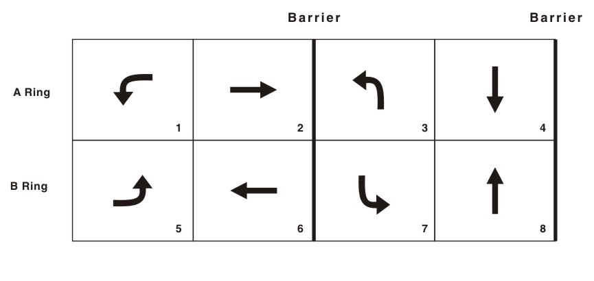
Phases: General Ideas Eight-phase, dual ring, NEMA controllers are often set up as shown in Exhibit 2-11. The diagram shows the movement sequences in the A and B rings. The green indications progress through the A and B rings simultaneously, in parallel, and the two barriers (between movements 2&6 and 3&7 and between movements 4&8 and 1&5) are crossed simultaneously in both rings.
The typical way in which the signal indications progress is as follows: greens are first displayed for movements 1&5, the eastbound and westbound protected lefts. These lefts lead the through movements assuming both are called. When actuations cease for either movement 1 or 5, for example movement 1 in this case, the green in the A Ring changes from movement 1 to movement 2, while movement 5 is still green. When movement 5 terminates, the green in the B ring changes from movement 5 to 6. An alternate sequence of distinct intervals can occur if the signal changes from 1&5 to 1&6 and then 2&6. Thus, the following phase sequences can occur left of the middle barrier: 1&5 to 1&6 to 2&6 (three intervals); 1&5 to 2&5 to 2&6 (again three intervals); 1&5 to 2&6 simultaneously (two intervals); 2&6 alone (1 and 5 both skipped). To the right of the barrier, four similar sequences are possible.
Discussion: to Skipped Phases |
Page Break
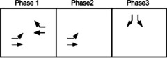
Sub-problem 1a: Maxwell Drive PM Peak Hour - Existing Conditions Skipped Phases: Consideration at Maxwell Drive At Maxwell Drive, the signal phasing is different from what’s shown in Exhibit 2-11. First, the eastbound left lags rather than leads the WB through (and right). Second, only movement 4 exists to the right of the middle barrier. The signal phasing is shown in Exhibit 2-12. When movement 5 is green, permissive EB lefts are allowed. If all of the lefts can turn while movement 5 is green, the 2&5 combination is skipped and the signal progresses from 1&5 directly to 4. If it’s not skipped, the sequence is 1&5, 2&5, and then 4.
The answer is that, if you're working from observational data alone, then you adjust the modeled signal timings so that they reflect an average cycle given that specific phase(s) will sometimes be skipped. In this case, phase 2 (see Exhibit 2-5) averages 10 seconds of green when it comes up, followed by a 3-second yellow and a 1-second all-red. Since the phase is skipped every other cycle, the signal timings you use in the HCM for this phase should be: 5 seconds of green, 1.5 seconds of yellow, and 0.5 seconds of all-red. to Skipped Phases |
Page Break
Sub-problem 1a: Maxwell Drive PM Peak Hour - Existing Conditions Skipped
Phase: What if skipped phases are ignored?
These three solutions also illustrate the huge variations in delay that can be achieved depending on the signal timings you use. It’s important to tell your client and the other stakeholders what signal timing philosophy you’re using so they know, or have some idea, what results to expect. Ideally, you’re using a philosophy that reflects what the signal will do in the field, but since that is heavily influenced by timing parameters employed (minimum greens, maximum greens, gap times and a host of other values), it’s hard to exactly duplicate the field performance. As an alternative to this observational approach, you might also consider applying one of the signal timing estimation procedures described in Chapter 16, Appendix B of the HCM. The decision on which approach is most appropriate depends on the available data, the required accuracy, and available time and resources.
|
|||||||||||||||||||||||||||||||||||||||||||||||||||||||||||||||||||||||||||||||||||||||||||||||||||||||||||||||||||||||||||||||||||||||||||||||||||
Page Break
Sub-problem 1a: Maxwell Drive PM Peak Hour - Existing Conditions Discussion: In problem 1, we've learned the effects of changing the arrival type, we’ve seen what differences in performance might exist if different sets of data are used for the same site, and we’ve seen what you should do to address skipped phases. More generally, we’ve seen that you need to be explicit in describing to the client how you’ve addressed these issues in establishing the base case results. Somebody else might get results that are quite different from yours, depending upon how they address these issues. You’ve got to be careful about the assumptions you make in correctly representing the conditions that exist in the field. to Sub-problem 1b |
Page Break
Sub-problem 1b: Maxwell Drive PM Peak Hour - With Conditions Let’s now explore some modeling issues in the context of the PM With conditions for the Maxwell Drive intersection. The intersecting volumes for both the PM Without and PM With condition are shown in Exhibit 2-14. We will focus on the PM With condition. It will be useful to see (by the differences) the traffic growth we’ve assumed between the base case volumes (Exhibit 2-7) and the PM Without conditions as well as the site-generated traffic we’ve added between the PM Without and the PM With conditions.
TEV: Total Entering Vehicles Analyses: |
||||||||||||||||||||||||||||||||||||||||||||||||||||||||||||||||||||||
Page Break
Sub-problem 1b: Maxwell Drive PM Peak Hour - With Conditions
Configuration Issues For Maxwell Drive, with
the new site traffic, we have an opportunity to see what designs will work
best. There isn’t going to be just one right answer; most likely, there
will be several. That’s usually the case with design problems. We’re going to start
by examining the volumes for the "with" condition (presented in
Exhibit
2-14), independent of what actually exists on the ground right now. For example, the
intersection was originally constructed wide enough to accommodate a
southbound through lane if a fourth leg were ever to be added to the
intersection. In the interim, the extra width has been used to accommodate
dual southbound left-turn lanes. But, are dual left-turn lanes really
going to be needed? The volumes suggest that we’re likely
to need at least one southbound left-turn lane, and maybe two. Two would
produce a per-lane match between the northbound and southbound lefts,
ignoring lane utilization. If we don’t use two, we might be able to
convert the second one into a through lane or a
through-and-something lane. Although the northbound lefts are not as
heavy (150) as the southbound lefts, they are significant. A left-turn
lane (opposing the southbound left-turn lane) would be wise. The through volumes are small both north and southbound.
That means one through lane should be plenty. We could even combine the throughs and rights. Now, let’s study lane configuration options. At the same time, we need to think about the signal timing plan. There are two tools to do this. One is the HCM planning method for signalized intersections. The other is critical lane analysis. It’s a simple, back-of-the-envelope technique for seeing what geometric/signal timing combinations might work. (The critical lane technique is discussed in most traffic engineering textbooks and handbooks, and it’s the method for signal timing presented in the HCM.) In each of these two analyses, we’re going to look at different lane configurations, phasing, signal timing, and cycle length. Acceptable cycle lengths range from 40-120 seconds, although longer and shorter values are possible.
Discussion: |
Page Break
Sub-problem 1b: Maxwell Drive PM Peak Hour - With Conditions
HCM Planning
Method For the Maxwell Drive, with the new site-generated traffic, Exhibit 2-15 presents the planning analysis results of nine model scenarios. Some show solutions that might be implemented in the field. Others show how the model thinks. In all scenarios, the peak hour factor is 0.94, the lost time per movement is 4 seconds (this is firm), there isn’t any coordination, there aren’t any parking maneuvers, the minimum cycle length is 10 seconds, and the maximum cycle length is 200 seconds. You can see the input data for Scenario P-1 in Dataset 9.
|
||||||||||||||||||||||||||||||||||||||||||||||||||||||||||||||||||||||||||||||||||||||||||||||||||||||||||||||||||||||||||||||||||||||||||||||||||||||||||||||||||||||||||||||||||||||||||||||||||||||||||
Page Break
Sub-problem 1b: Maxwell Drive PM Peak Hour - With Conditions Scenario P-1 is a good place to start our discussion. It represents a legitimate option. The left turns are protected and the lanes are configured in a logical way. (If there are no right- or left-turn lanes, the model assumes the movements are shared with the through movement.) Let's conduct some "what-if" analyses that go beyond the results and data sets presented in the previous Exhibit.
The model estimates a cycle length of 171.4 seconds (for a condition where
cycle length is the minimum possible). That’s too long. If the number of
northbound and southbound through lanes is increased to 3, as in Scenario
P-2, nothing happens. That’s because the through movement is not the
critical movement, and so it does not determine the cycle length. If you
reconfigure the north and southbound approaches so there are two left-turn
lanes and one through-and-right lane, the cycle length drops to 104.5
seconds. This is better, but it assumes it's possible to have simultaneous
opposing dual lefts, which isn’t allowed in New York State. If permissive
lefts are assumed, the model drops the cycle length to 18.5 seconds. That’s
too short for most practical situations. The model is reporting the shortest
cycle length that puts the intersection at capacity using the equations used
to set the signal timings. A more practical value, like 80 seconds, makes
the model show that the intersection is under capacity for that cycle
length. At a cycle length of 20 seconds, the model shows the intersection is
near capacity and, with cycle lengths of 25 seconds or above, it shows the
intersection operating under capacity.
Now we’ll do some sensitivity analyses, mostly
to illustrate trends. If we assume dual lefts northbound and southbound,
along with exclusive lanes for the throughs and rights, the cycle length
drops to 76.5 seconds (from the previous 104.5). If we add dual lefts and
three through lanes eastbound and westbound, the cycle length drops to 38.5
seconds.
If we take that same lane configuration and consider a more reasonable cycle
length, say 45 seconds, the model shows the intersection is near capacity.
If we go back to single left-turn lanes northbound and southbound, the model
calculates a cycle length of 53.5 seconds.
Discussion: |
Page Break
Sub-problem 1b: Maxwell Drive PM Peak Hour - With Conditions
Cycle Length
Education
where vi is the volume for the critical movement in phase i, si is the saturation flow rate for the critical movement in phase i, N is the number of phases per cycle, and L is the lost time per phase. For actuated signals
with dual-ring controllers like the one we portrayed in
Exhibit 2-11, it
helps to expand Equation (1) into three equations. The first one computes
the v/s ratio for sequential pairs of movements to the left
and right of the middle barrier in the A and B rings
Here pq takes on the values 1&2, 3&4, 5&6, and 7&8 corresponding to the four quadrants of the dual ring pattern. The second equation computes the maximum v/s ratio for the left and right halves of the dual ring pattern:
The third equation takes the two results from Equation (3) and computes a minimum cycle length:
Equations (2) through (4)
show that Equation (1) can
be obtained easily. First, realize that N equals 4.
Second, see that the sequence of critical movements is either:
1,2,3,4; 1,2,7,8; 5,6,3,4; or 5,6,7,8. Third, notice that the
sum of the vi/si ratios identified in
the denominator of Equation (1) is the same as the left and
right half based sum shown in Equation (4).
|
Page Break
Sub-problem 1b: Maxwell Drive PM Peak Hour - With Conditions Critical Movement
Technique
Exhibit 2-16 shows the
results that were obtained using the critical lane analysis for eight
different scenarios. We have assumed that the
saturation flow rates for the various
lane groups are as indicated by the note below the table and that the
lost time per phase is as shown in the second column. |
Page Break
Sub-problem 1b: Maxwell Drive PM Peak Hour - With Conditions Discussion: |
Page Break
Sub-problem 1b: Maxwell Drive PM Peak Hour - With Conditions
What have we learned from this? We’ve seen that we can make the signal work, in an operational analysis, for the conditions that the planning analyses suggested should work. We have also seen that the cycle lengths are sometimes different. One final observation is that it seems possible with the operational analysis to fine-tune the problem solution in some cases so that better than at-capacity performance can be achieved through careful selection of the phasing plan and the lane configuration. |
||||||||||||||||||||||||||||||||||||||||||||||||||||||||||||||||||||||||||||||||||||||||||||||||||||||||||||||||||||||||||||||||||||||||||||||||||||||||||
Page Break
Sub-problem 1b: Maxwell Drive PM Peak Hour - With Conditions
Uncertainty Issues
For this particular intersection, let’s look at three situations: the base
case (Dataset 10),
a condition with 30% more site-generated traffic (Dataset
13), and a condition with 30% less site generated traffic (Dataset
14).
The results are presented in Exhibit 2-18. It’s
interesting that increasing the site-generated volumes by 30% raises the
cycle length substantially from 65 to 77 seconds. The delays also increase
from an average of 28.7 seconds to 34.4 seconds. However, when the
site-generated traffic is lower by 30% there isn’t a significant change.
The cycle length stays at 65 seconds, the average delay drops only
marginally from 28.7 to 28.5 seconds.
It’s hard to see the trends in delays, etc. directly from the table. A graphic is useful. Exhibit 2-19 shows a radar plot of the delay trends. Each axis of the wheel is used to present the delay for a given movement. The lines and symbols show the delay for a given scenario. All five operational solutions discussed in Exhibit 2-17 and Exhibit 2-18 are included. If you look at the plots for C-4 (the base case) and Datasets 11 and 12, that trend is clear. The pattern for Dataset 11 is outside the pattern for C-4, which makes sense since the site traffic volumes for Dataset 11 are 30% greater than for C-4. The pattern for Dataset 12 is inside the pattern for C-4 for a similar reason. The site-related traffic is 30% less than in C-4. The patterns for scenarios C-7 and C-8 are different. Most notably, in both of those scenarios there are more lanes available for the northbound and southbound lefts. In C-7, we’ve provided two left-turn lanes on both approaches. In C-8, there are three lanes being shared among the lefts, throughs, and rights, both northbound and southbound. As a result, the SL delays in particular, and the NL delays to a lesser extent, are noticeably smaller than they otherwise might be if the extra lane capacity had not been provided (i.e., the pattern in C-4 would have still applied). |
||||||||||||||||||||||||||||||||||||||||||||||||||||||||||||||||||||||||||||||||||||||||||||||||||||||||||||||||||||||||||||||||||||||||||||||||||||||||||||||||||||||||||||||
Page Break
|
Exhibit 2-19. Maxwell Drive Delay Patterns among Scenarios
|
Page Break
Problem 1: Maxwell Road
Discussion We haven’t presented
all of the analyses that would be required to do a complete traffic impact
assessment. Rather, we’ve used certain conditions to illustrate
important ideas related to the use of the HCM. We’ve used the PM
Existing condition to look at arrival patterns, skipped phases, and
differences in LOS stemming from the use of data from different sources.
We’ve used the PM With condition to look at changes in LOS due to the
addition of the site-related traffic, the relationship between geometric
improvements and LOS, differences between planning and operational
analyses, and the role of uncertainty in affecting the results obtained. We don’t know for
sure that the new configuration we’ve identified is the best.
We’ve focused only on the PM With condition. It’s possible that the AM
With or some other condition would work better with some other
configuration. That’s something you’d have to do to complete the impact assessment. |